Background
Recently I saw that Google was offering curated career certificates and there was one for Data Anaytics, so I decided I’d check it out and see what the programs are like (check out my certificate here). Maybe I’ll post about it later, but for now this is a case study from the certificate program that uses anonymized data from biekshare rides in Chicago in 2020. It’s formatted more like an actual report than other projects I’ve shared.
Business Task
In order to better convert casual riders into members, we need to determine the major differences between the two and how these differences can be overcome; specifically in relation to social media.
Preparing The Data
The raw data is split into several .csv files. Each file represents one month from 04/2020 to 12/2020, with one .csv file containing all of the 2020Q1 data (01/2020 - 03/2020). To prepare the data for easier processing, I moved all the .csv files to a subfolder on Google Cloud Storage labeled “raw_data” inside a “case_study_data” folder. Each .csv file has the following columns:
ride_id, rideable_type, started_at, ended_at, start_station_name, start_station_id, end_station_name, end_station_id, start_lat, start_lng, end_lat, end_lng, member_casual
After cleaning, the files were uploaded to a Google Cloud Storage bucket “cleaned_case_study_data” in the “case_study_data” bucket.
Data Processing
The data was mostly clean and intact. Later dates have missing station info, but I kept these records in the dataset anyway because they still had member and other ride information. The file for 12/2020 was the biggest issue: it had incorrect start and end station IDs which were also strings instead of doubles. I used XLOOKUP() in excel to fix these using the station names where available.
After addressing any data errors, I uploaded the files to BigQuery and created a table that includes all records to go along with the monthly files, called cleaned_all_ride_data_2020.
I inserted an INT64 column called “ride_length” into the aggregated ride table then ran:
UPDATE data_case_study.all_ride_info_2020

SET ride_length = DATETIME_DIFF(ended_at, started_at, SECOND)

WHERE ended_at IS NOT NULL
Then I added another INT64 column named day_of_week and used:
UPDATE data_case_study.all_ride_info_2020

SET day_of_week = EXTRACT(DAYOFWEEK FROM started_at)

WHERE ended_at IS NOT NULL
to fill it with the day each ride was made (1-7, with 1 being Sunday). There is the possibility of an edge case where a user ordered the bike one day and returned it the next (perhaps from 11:30pm to 2:30am for example), but I think using the start_date as the whole transaction’s weekday makes the most sense because that is the day the user made the choice to rent, regardless of return date.
After combining files and running a few queries I realized there was an issue which would make visualization hard: the station coordinates were not consistent length, which would lead to one station having different map locations. I decided the fastest way to fix this was just to make a new table by saving the following query results:
SELECT ride_id,

  rideable_type,

  started_at,

  ended_at,

  COALESCE(start_station_name, 'No Station') AS cleaned_start_station_name,

  start_station_id,

  MAX(start_lat) OVER (PARTITION BY start_station_name) AS cleaned_start_lat,

  MAX(start_lng) OVER (PARTITION BY start_station_name) AS cleaned_start_lng,

  COALESCE(end_station_name, 'No Station') AS cleaned_end_station_name,

  end_station_id,

  MAX(end_lat) OVER (PARTITION BY end_station_name) AS cleaned_end_lat,

  MAX(end_lng) OVER (PARTITION BY end_station_name) AS cleaned_end_lng,

  member_casual,

  ride_length,

  day_of_week

FROM data_case_study.all_ride_info_2020
An obvious caveat of this query is that it will give all the NULL station names the same coordinates. However, there were only about 600 distinct values falling into this category, and they were all two decimal places or less (accuracy up to within about 1Km). Since they were also only within less than a degree of each other, I decided they were not accurate enough to provide more detail than the city anyways, and so were not worth dealing with individually. These points will simply be excluded from any map visualization, but will still be kept for ride length, member info, etc. I gave these the “No Station” title for easier use later.
I also noticed there were a few stations with names but NULL ID numbers. There are 600+ station names and there were several thousand of these NULL ID situations with actual location names. Because of the number of instances CASE statements were not feasible. Window functions were a choice but the only way I could think to get that to work would be to use LAG and order DESC or something, or to use AVG (since NULL is not included in AVG and thus would return just the correct ID number), but these both felt sort of hacky, especially the window function option. Since I couldn’t figure out a reasonable way to do this in SQL and I don’t plan on using the ID numbers for much anyways, I decided to just leave the NULL ID values intact (this is also why the coordinates are partitioned over names; there were no IDs without a name but plenty of names without an ID).
Analysis
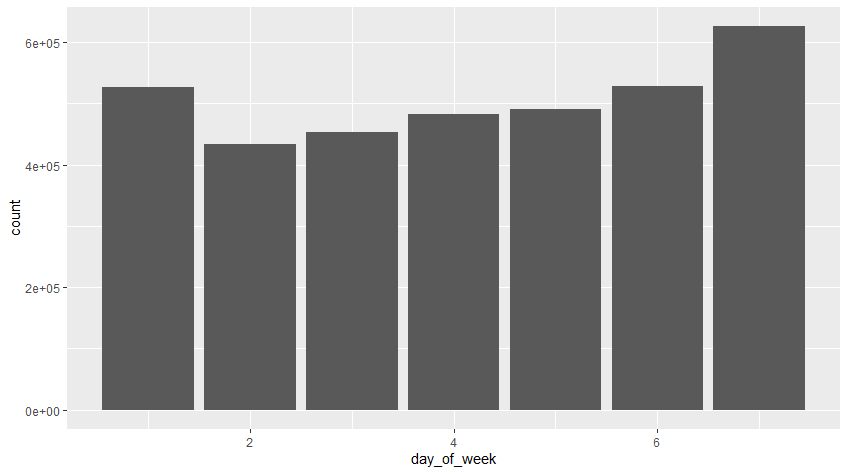
First I wanted to check if there are any days that stick out for high or low use. I ran a simple SQL query to get weekends vs weekdays to start. There were 1,153,399 rides on weekends and 2,388,284 rides on weekdays. Clearly weekends represent a slightly higher proportion of rides (weekends are 29% of the week but 33% of rides). Let’s drill deeper into this.
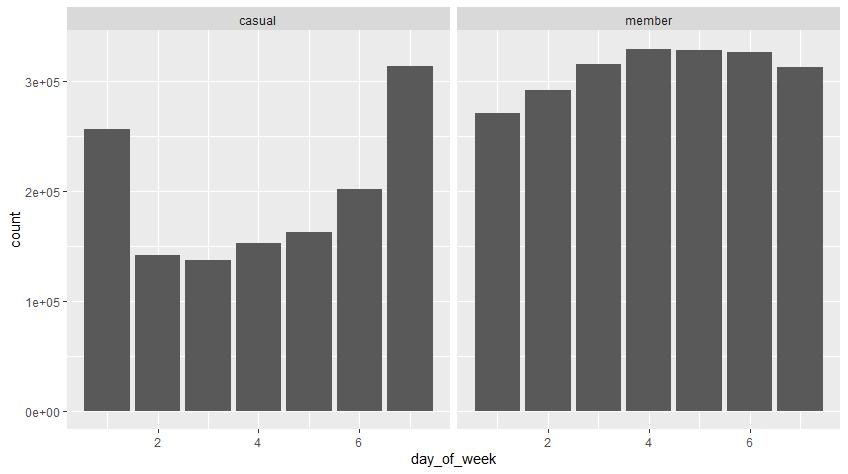
Of all weekend rides, 569,951 were done by “casual” users, representing 49% of weekend users. In comparison, weekday rides only have 796,624 total “casual” riders, representing 33% of that total. It seems that casual riders are most likely to be weekend users. Finally, let’s see how long the casual weekend users’ rides are compared to members. Casual users average a ride length of 3060 seconds (51 minutes) while members average only 1075 seconds (a little under 18 minutes). For weekdays it’s 2509 vs 569 (just under 42 minutes vs 9.5 minutes). So it seems casual users use the bikes for significantly longer times than members. Indeed, looking at total weekday ridership times for 2020, members rode a cumulative 15,107,517 minutes while casual riders rode 33,319,282 minutes. Let’s keep this in mind, and look at member specific information.
As we know, members are most likely to use a bike during the weekday for only about 10 minutes. This might be a matter of them using bikes for a commute or for other short yet regular trips (like grocery shopping). Let’s see if there are any stations that get a particularly high usage during the week.
SELECT start_station_name, COUNT(start_station_name) AS station_rides

FROM data_case_study.all_ride_info_2020

WHERE day_of_week IN (7, 1) AND member_casual = 'member'

GROUP BY start_station_name

ORDER BY station_rides DESC
This doesn’t return any clear results: there aren’t any stations that have significantly more rides than the others. However, comparing start and end station data, a couple stations are in the top for both. This would suggest there’s a high number of members riding between them on the same day. Additionally, there is little to no overlap between top weekday start/end stations for members and those for casual users.
Back to the differences in ride length. Casual users are actually prolific users of Cyclistic bikes, especially during weekends. Weekdays in particular are worth investigating more though, as casual users make up a minority of the rental instances, but a large majority of the rental time. The Streeter Dr. and Grand Ave and the Lakeshore and Monroe locations are the two top start/end destinations and are in close proximity to miles of waterfront parks and walking/bike paths. Looking into these locations further, most rides starting or ending there are round trip rides. This trend suggests that casual users are taking bikes for a ride along the waterfront which would explain the long rentals and the round trip pattern. If it was tourist usage to the pier and Magnificent Mile, I’d expect round trips to be rare as people are transiting from a hotel then walking around before heading back from a different rental location. Likewise, commutes would obviously not be round trip rides. This pattern continues to hold true over the weekend.
Finally, there’s a difference in bike types that’s worth looking into. There are classic bikes, docked bikes, and electric bikes. Unfortunately, there were no real insights in this data. I initially assumed there might be a preference for docked bikes among members and electric bikes among casual users, but in reality the different groups use each bike type at about the same rate.
Visualizations
For this project I decided to use R for visualizations instead of Tableau. If I was more comfortable with R I also would have used it for the other steps, but I’m not quite there yet. There are just a couple to clarify a main point, this project was mostly focused on analysis.
First we have number of rides per day:

As mentioned before, there’s a clear preference for weekends, and again we see this is driven by casual users:

Conclusion
There are two major differences between members and casual users. One, casual users are much more likely to use a bike on a weekend vs a weekday, while it’s the opposite for members. Two, casual users spend a significantly longer time on the bikes as opposed to members. This suggests that members are using the bikes to commute and run quick errands while casual users are using them for leisure.
Recommendations
In order to convert casual users to members, I recommend focusing advertising and other changes on the difference in usage. For example, target advertising to casual users during long weekends, holidays, or events in the park (when they are likely to be using a bike already) extolling the benefits of a membership vs one time rentals. Another option might be to add more bikes in the park which will facilitate more rides for casual users, thereby making them more likely to sign up for a membership to make it easier to take advantage of the increased bike availability. Another possibility is targeting advertisements at non members explaining the benefits of commuting with the bikes. Since commuters are more likely to be members, casual users that are comfortable renting bikes already can be converted into regular users and therefore members. Finally, it could be worthwhile to create a new membership tier that is only for weekends, or is available in hour-long blocks (at a slight discount from the per minute price of an equivalent ride), to spur casual users to become members in order to realize perceived rental cost savings.